Back التنبؤ الرقمي للطقس Arabic Model numèric de predicció meteorològica Catalan Numerische Wettervorhersage German Αριθμητική πρόγνωση καιρού Greek Cifereca veterprognozo Esperanto Modelo numérico de predicción meteorológica Spanish پیشبینی عددی وضع هوا Persian Numeerinen säänennustaminen Finnish Prévision numérique du temps French Numerikus időjárás-előrejelzés Hungarian

Numerical weather prediction (NWP) uses mathematical models of the atmosphere and oceans to predict the weather based on current weather conditions. Though first attempted in the 1920s, it was not until the advent of computer simulation in the 1950s that numerical weather predictions produced realistic results. A number of global and regional forecast models are run in different countries worldwide, using current weather observations relayed from radiosondes, weather satellites and other observing systems as inputs.
Mathematical models based on the same physical principles can be used to generate either short-term weather forecasts or longer-term climate predictions; the latter are widely applied for understanding and projecting climate change. The improvements made to regional models have allowed significant improvements in tropical cyclone track and air quality forecasts; however, atmospheric models perform poorly at handling processes that occur in a relatively constricted area, such as wildfires.
Manipulating the vast datasets and performing the complex calculations necessary to modern numerical weather prediction requires some of the most powerful supercomputers in the world. Even with the increasing power of supercomputers, the forecast skill of numerical weather models extends to only about six days. Factors affecting the accuracy of numerical predictions include the density and quality of observations used as input to the forecasts, along with deficiencies in the numerical models themselves. Post-processing techniques such as model output statistics (MOS) have been developed to improve the handling of errors in numerical predictions.
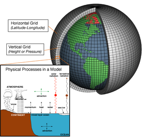
A more fundamental problem lies in the chaotic nature of the partial differential equations that describe the atmosphere. It is impossible to solve these equations exactly, and small errors grow with time (doubling about every five days). Present understanding is that this chaotic behavior limits accurate forecasts to about 14 days even with accurate input data and a flawless model. In addition, the partial differential equations used in the model need to be supplemented with parameterizations for solar radiation, moist processes (clouds and precipitation), heat exchange, soil, vegetation, surface water, and the effects of terrain. In an effort to quantify the large amount of inherent uncertainty remaining in numerical predictions, ensemble forecasts have been used since the 1990s to help gauge the confidence in the forecast, and to obtain useful results farther into the future than otherwise possible. This approach analyzes multiple forecasts created with an individual forecast model or multiple models.